Euclidean vs Manhattan Distance

Python
import matplotlib.pyplot as plt
import numpy as np

# Define two points
p1 = (1, 2)
p2 = (7, 6)

# Calculate distances
euclidean_distance = np.sqrt((p2[0] - p1[0])**2 + (p2[1] - p1[1])**2)
manhattan_distance = abs(p2[0] - p1[0]) + abs(p2[1] - p1[1])

# Create the plot
plt.figure(figsize=(8, 8))
plt.grid(True, linestyle='--', alpha=0.6)
plt.axhline(0, color='black',linewidth=0.5)
plt.axvline(0, color='black',linewidth=0.5)

# Plot points
plt.plot(p1[0], p1[1], 'ro', markersize=10, label=f'Point 1 ({p1[0]}, {p1[1]})')
plt.plot(p2[0], p2[1], 'bo', markersize=10, label=f'Point 2 ({p2[0]}, {p2[1]})')

# Plot Euclidean distance (straight line)
plt.plot([p1[0], p2[0]], [p1[1], p2[1]], 'g-', label=f'Euclidean Distance = {euclidean_distance:.2f}')

# Plot Manhattan distance (city block path)
plt.plot([p1[0], p2[0], p2[0]], [p1[1], p1[1], p2[1]], 'm--', label=f'Manhattan Distance = {manhattan_distance}')
# Alternative Manhattan path for visualization
# plt.plot([p1[0], p1[0], p2[0]], [p1[1], p2[1], p2[1]], 'y--')


# Set plot limits and labels
plt.xlim(0, 8)
plt.ylim(0, 8)
plt.xlabel("X-axis")
plt.ylabel("Y-axis")
plt.title("Euclidean vs. Manhattan Distance")
plt.legend()
plt.gca().set_aspect('equal', adjustable='box')
plt.savefig("distance_comparison.png")
plt.close()
Of course, let’s break down the differences between Euclidean and Manhattan distance with a visual explanation and their applications.
The Core Difference
The fundamental difference lies in how “distance” is measured between two points.
- Euclidean distance is the most intuitive and common way we think of distance. It’s the straight-line path between two points, as if you could travel directly “as the crow flies.” 🐦
- Manhattan distance, also known as “city block” or “taxicab” distance, is the distance you would travel between two points if you were restricted to moving along a grid. Imagine walking in a city like Manhattan, where you have to follow the streets (north-south and east-west) to get from one point to another. 🚕
Visual Comparison
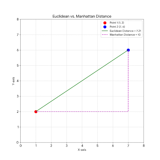
The graph below illustrates the difference. We have two points, Point 1 at (1, 2) and Point 2 at (7, 6).
![Euclidean vs. Manhattan Distance]()
- The green line represents the Euclidean distance. It’s the shortest, most direct path between the two points.
- The purple dashed line shows one possible path for the Manhattan distance. To get from Point 1 to Point 2, you must travel along the grid lines, first horizontally and then vertically. The total length of this path is the Manhattan distance.
Formulas and Calculation
Let’s consider two points, P_1 at (x_1,y_1) and P_2 at (x_2,y_2).
Euclidean Distance
The formula is derived from the Pythagorean theorem:
Distance=(x2−x1)2+(y2−y1)2
For our example points (1, 2) and (7, 6):
Distance=(7−1)2+(6−2)2=62+42
=36+16
=52
≈7.21
Manhattan Distance
The formula is the sum of the absolute differences of the coordinates:
Distance=∣x2−x1∣+∣y2−y1∣
For our example points (1, 2) and (7, 6):
Distance=∣7−1∣+∣6−2∣=∣6∣+∣4∣=6+4=10
As you can see, the Manhattan distance is always greater than or equal to the Euclidean distance.
Applications
The choice between Euclidean and Manhattan distance depends entirely on the context of the problem you are trying to solve.
Applications of Euclidean Distance
This is used when movement is not restricted to a grid.
- Physics and Engineering: Calculating the trajectory of projectiles or the distance between objects in space.
- Computer Graphics: Determining the distance between objects in a 3D scene for lighting and collision detection.
- Machine Learning: In algorithms like K-Nearest Neighbors (KNN), it’s a common way to measure the “closeness” of data points in a feature space.
Applications of Manhattan Distance
This is ideal for scenarios where movement is constrained to a grid or a stepwise path.
- Urban Planning and Logistics: Calculating travel times or distances in cities with a grid-based street layout. This is why it’s called “taxicab distance.”
- Chess and other Board Games: Determining the minimum number of moves a piece like a rook needs to get from one square to another. ♟️
- Image Processing: Measuring the difference between pixels, where you can only move from one pixel to an adjacent one.
- Bioinformatics: It can be used in comparing DNA sequences.
Share this content:


Post Comment